

Autonomous Space Robotics Lab
Gravel Pit
Lidar-Intensity Imagery Dataset
[Overview] [Hardware Setup] [Datasets] [Data Description] [Tools] [Credits] [Acknowledgements]

Overview
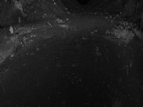
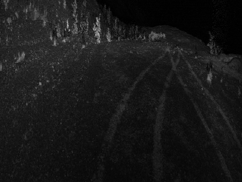
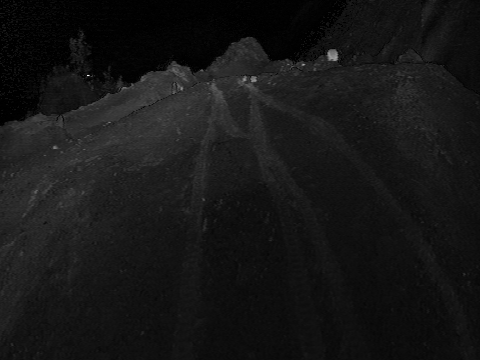
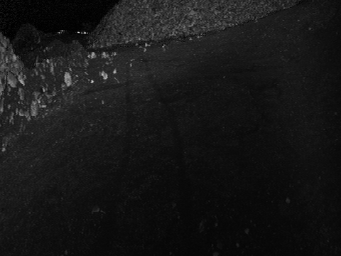
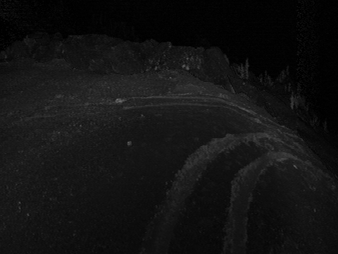
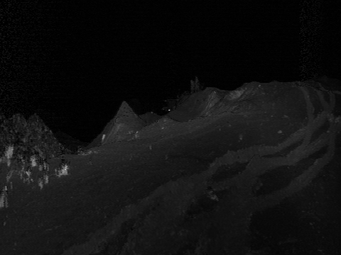
The Gravel Pit Lidar Intensity Imagery Dataset is a collection of 77,754 high-framerate laser range and intensity images gathered at a suitable planetary analogue environment in Sudbury, Ontario, Canada. The data were collected during a visual teach and repeat experiment in which a 1.1km route was taught and then autonomously re-traversed (i.e., the robot drove in its own tracks) every 2-3 hours for 25 hours. The dataset is subdivided into the individual 1.1km traversals of the same route, at varying times of day (ranging from full sunlight to full darkness).
This data should be of interest to researchers who develop algorithms for visual odometry, simultaneous localization and mapping (SLAM) or place recognition in three-dimensional, unstructured and natural environments. In concert with state-of-the-art techniques, this dataset creates ample opportunity for loop closure; in addition to having multiple traversals of the same path, the trajectory was specifically chosen to include both small- and large-scale loops. The lidar scans were taken with a $480 \times 360$ resolution at 2Hz, while driving roughly 0.3-0.4 meters per second; therefore, one of the challenges in using this dataset is to compensate for the motion distortion in the data. All of the data are presented in either human-readable text files or images, and are accompanied by Matlab parsing scripts for ease of use.

Hardware Setup
The robuROC 6 used to gather the dataset carried a number of payloads. The relevant payloads for this dataset consisted of a high-framerate Autonosys LVC0702 lidar, and a Thales DG-16 Differential GPS unit.
The Autonosys LVC0702 lidar provides 500,000 measurements per second with a 15-bit intensity at a maximum range of ~53.5m. In this dataset, the lidar was configured to have a 90°H/30°V FOV, and capture images with a resolution of 480x360 at 2Hz.
The Thales DG-16 Differential GPS unit has a Circular Error Probability (CEP) of 0.4m, with 95% of measurements occuring within 0.9m.
Overview of Datasets
Each of the entries below contain data products related to a unique traversal of the 1.1km route (conducted at different times of day). For ease of use, the data has been post-processed and packaged into a few different products. The Header .zip file contains general dataset information, including the GPS tracks and a few alignment matrices.
The first major data product, Imagestacks, contains a sequence of images, generated from the raw sensor data, in the Tagged Image File Format (TIFF). Each intensity image in the sequence is accompanied by a corresponding azimuth, elevation, range and timestamp image. TIFF was chosen as it is supports both 32- and 64-bit floating point images. Also, TIFF is simple to load using either Matlab, or OpenCV, which leverages LibTiff (link).
The second major data product, SURF and Matches, contains a set of sparse SURF features extracted using the ASRL GPU accelerated SURF implementation (link). The sparse measurements are then corrected using the supplied calibration model (see the autonosys_apply_calib helper function). Finally, two sets of frame-to-frame matches are provided. The first set of matches are simply the initial guesses based on only the SURF descriptor. The second set of matches are the inliers after a being passed through a RANSAC algorithm that accounts for the motion distortion in the image.
In summary, the available downloads are:
Downloads
To start, it is recommended that the user download either the sample dataset (.zip [189 MB]), or the Header and Imagestacks for the 'teach 1' dataset, and get a feel for the data by using some of the example visualization code available in the Helpful Tools. The sample set consists of typical data collected over 30 meters of traversal (including both straight motion and a gradual turn).
Important note: The dataset provides ftp download links. Some browsers no longer enable ftp links by default and you need to change the settings if you want to download using the browser. Using the wget command is an alternative to avoid the browser.
| Traverse | # of Frames | Start Time | End Time | Video | Header | Imagestacks | SURF and Matches |
|---|---|---|---|---|---|---|---|
| teach 1 | 6880 | 19:45:xx | xx:xx:xx |
|
.zip [155 KB] |
.zip [10.0 GB] |
.zip [1.3 GB] |
| run 1 | 7039 | 23:03:27 | 00:03:39 |
|
.zip [159 KB] |
.zip [10.2 GB] |
.zip [1.3 GB] |
| run 4 | 6741 | 05:00:28 | 05:56:26 |
|
.zip [119 KB] |
.zip [9.7 GB] |
.zip [1.3 GB] |
| run 5 | 8679 | 09:47:12 | 10:57:13 |
|
.zip [159 KB] |
.zip [12.4 GB] |
.zip [1.5 GB] |
| run 6 | 9694 | 11:51:36 | 13:20:19 |
|
.zip [209 KB] |
.zip [13.6 GB] |
.zip [1.8 GB] |
| run 7 | 9644 | 14:15:54 | 15:35:51 |
|
.zip [206 KB] |
.zip [13.9 GB] |
.zip [1.6 GB] |
| run 8 | 8691 | 16:25:05 | 17:32:41 |
|
.zip [162 KB] |
.zip [12.4 GB] |
.zip [1.6 GB] |
| run 9 | 6456 | 18:24:19 | 19:18:41 |
|
.zip [146 KB] |
.zip [9.4 GB] |
.zip [1.2 GB] |
| run 10 | 7863 | 20:31:06 | 21:37:36 |
|
.zip [175 KB] |
.zip [11.2 GB] |
.zip [1.5 GB] |
| run 11 | 6067 | 22:58:43 | 23:50:06 |
|
.zip [139 KB] |
.zip [8.7 GB] |
.zip [1.1 GB] |
Additional Notes
Description of Data Products
In this section, we detail the format of the data in addition to specifics such as experimental considerations and post-processing details. Each traverse dataset consists of a series of folders corresponding to the various data producs. These folders contain either TIFF images or comma-delimited human-readable text files.
Coordinate Frames
For clarity, we provide an image below illustrating the various coordinate frames that relate to the measurement data.

The three frames in the image above are the sensor frame,  , the GPS frame,
 , and the inertial frame,
  .
This dataset uses homogeneous transformation matrices to express the translation and rotation between frames.
For example, to transform a 3D point from
.
This dataset uses homogeneous transformation matrices to express the translation and rotation between frames.
For example, to transform a 3D point from  to
to  , a transformation matrix,
 , may be used in the following manner:
where  is the vector from to point
  , expressed in ,
 is the vector from to point , expressed in ,
 is the rotation matrix from to ,
and
is the rotation matrix from to ,
and  is the translation from to , expressed in .
The first matrix we provide is the 4x4 homogeneous transformation matrix relating the sensor frame and GPS frame. For simplicity and due to the scale of the CEP, this transform is assumed static, and provided only for the nominal position of the pods. Second, each traverse dataset contains a transformation matrix to bring the initial local GPS frame into angular alignment with the inertial GPS data. This alignment matrix is calculated by performing a simple point-to-point least-squares optimization between the first 30 meters of our visual odometry estimate and the GPS data.
The file format for matrices, matrix_<name>.txt, is straight forward. The first line contains the comma separated number of rows and columns in the matrix. The following lines contain the floating-point data of the matrix (comma separated for columns and and line separated for rows).
Dataset Header File
The header file is a human-readable, comma-delimited text file with information pertaining to the contents of the dataset. There is a single header line in the file to describe the contents of each data column. The following shows the file naming convention and more detailed descriptions of the contained items:
<dataset-name>_header.txtGPS Data File
The GPS data file is a human-readable, comma-delimited text file containing the GPS coordinate at each frame capture. During the collection phase, the GPS and camera were not synchronized. To account for this, the GPS coordinates that are provided have been interpolated from the original data using the timestamp at each frame.
There is a single header line in the file to describe the contents of each data column. The following shows the file naming convention and more detailed descriptions of the contained items:
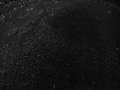
<dataset-name>_gps.txtImage Stack

|

|
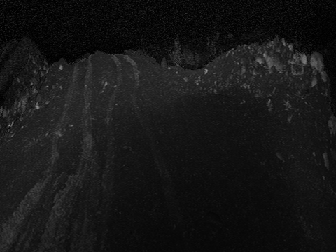
| Example Intensity Image | Example Range Image |
For each frame listed in the header file, there exists a set of .tif images that make up a single image stack. Images of different types are separated and named accordingly:
img_azimuth/<dataset-name>_<id>_img_azimuth.tif - 32-bit floating point azimuth angle (radians)img_elevation/<dataset-name>_<id>_img_elevation.tif - 32-bit floating point elevation angle (radians)
img_range/<dataset-name>_<id>_img_range.tif - 32-bit floating point range measurement (meters)
img_time/<dataset-name>_<id>_img_time.tif - 64-bit floating point time (seconds since beginning of experiment)
img_intensity16/<dataset-name>_<id>_img_intensity16.tif - 16-bit raw intensity measurement
img_intensity8/<dataset-name>_<id>_img_intensity8.tif - 8-bit intensity measurement (range corrected)
img_mask/<dataset-name>_<id>_img_mask.tif - 8-bit mask image to identify missing pixel data (0-bad, 255-good)
|
The raw azimuth, elevation and range images make up the geometric portion of the scans and the associated spherical camera model is depicted below. Note that these raw measurements do not yet include the intrinsic calibration, which was performed using the generalized distortion model presented by Dong et al, in "Two-axis Scanning Lidar Geometric Calibration using Intensity Imagery and Distortion Mapping". The undistortion function is straight forward and has been made available in the Matlab code. Note that TIFF was chosen as it is supports both 32- and 64-bit floating point images. Additionally, TIFF is simple to load using either Matlab, or OpenCV, which leverages LibTiff (link). |

|
SURF Feature File

|

|
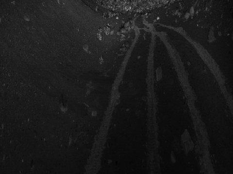
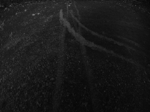
| Example SURF Features (Matches in Frame 1) | Example SURF Features (Matches in Frame 2) |
The SURF feature files contain a list of SURF features extracted from the Autonosys lidar intensity data. There is one SURF feature file for every image stack in the dataset. When using the sub-pixel (u,v) coordinate to extract measurements from the image stacks, the four surrounding pixels were used for bilinear interpolation. Additionally, the azimuth, elevation and range measurements have been idealized using the supplied calibration model (see the autonosys_apply_calib helper function).
There is a single header line in the file to describe the contents of each data column. The following shows the file naming convention and more detailed descriptions of the contained items:
<dataset-name>_<id>_surf.txtFeature Match File
The feature match file contains a list of indices that relate SURF features in sequential frames. Two types of match files have been provided. The first are the raw matches, which are based solely on the SURF feature descriptors. The second are the filtered matches, which provide only 'inlier' matches based on a RANSAC algorithm that accounts for motion distortion.
There is a single header line in the file to describe the contents of each data column. The following shows the file naming convention and more detailed descriptions of the contained items:
<dataset-name>_<id-A>_<id-B>_<matches-name>.txtHelpful Tools
The following tools are provided to assist in utilizing the data.
Matlab Functions/Scripts
- abl_load_header.m - Parses the dataset header file.
- abl_load_gps.m - Parses the dataset GPS file.
- abl_load_frame_imgstack.m - Loads an imagestack for a particular frame from the TIFF images.
- abl_load_frame_surf.m - Parses the SURF features for a particular frame.
- abl_load_matches.m - Parses the SURF feature matches for a particular set of frames.
- abl_load_matrix.m - Parses a dataset matrix file (such as a transformation matrix).
- abl_display_imagestack.m - A plotting function to show an imagestack.
- abl_display_surf.m - A plotting function to draw show features on the intensity image.
- abl_display_tracks.m - A plotting function to show feature tracks (matches) between images.
- autonosys_apply_calib.m - Uses the ASRL Autonosys calibration model to idealize raw measurements by correcting for some measurement distortions. This is conceptually similar to the image rectification process in computer vision. Note that this has already been applied to the SURF measurements in the dataset, but not to the imagestacks.
- autonosys_covariance.m - Spherical covariances used for the Autonosys lidar.
- autonosys_SphericalFromPoint.m - Ideal spherical camera model used for the Autonosys lidar.
- autonosys_PointFromSpherical.m - Ideal inverse spherical camera model used for the Autonosys lidar.
- example1_view_imgstacks.m - Example script that opens and displays the image stack.
- example2_view_matches.m - Example script that displays the feature tracks using the intensity imagery, SURF features and matches.
- example3_estimation.m - Example script for setting up an estimation problem. This only requires data from the second data product (SURF features and matches).
Credits
This dataset was the work of Sean Anderson, Colin McManus, Hang Dong, Erik Beerepoot and Timothy D. Barfoot. If you use the data provided by this website in your work, please use the following citation:
Anderson A, McManus C, Dong H, Beerepoot E, and Barfoot T D. “The Gravel Pit Lidar-Intensity Imagery Dataset”. University of Toronto Technical Report ASRL-2012-ABL001. (pdf)
Acknowledgements
The collection of this data would not have been possible without the support of many people. In particular, we would like the thank the staff of the Ethier Sand and Gravel in Sudbury, Ontario, Canada for allowing us to conduct our field tests on their grounds and Dr. James O'Neill from Autonosys for his help in preparing the lidar sensor for our field tests. We also wish to thank DRDC Suffield, MDA Space Missions, the NSERC, the Canada Foundation for Innovation and the Canadian Space Agency for providing us with the financial and in-kind support necessary to conduct this research.